Introduction
In this article, we describe how to perform kinetic analysis, equilibrium analysis, and concentration analysis of surface plasmon resonance (SPR) data on the ProteOn™ XPR36 system differential window. We also present details on how to customize sensorgram appearance and judge the quality of SPR results. Options for dataset export using the ProteOn Manager™ software are also included.
Kinetic Analysis
To determine the kinetic constants of a label-free biomolecular interaction through SPR analysis (described in detail in the Applications & Technologies section of the Bio-Rad website), the sensorgram must be fitted to a kinetic model using a mathematical algorithm. In ProteOn Manager software, the user may choose among seven different binding models with which to perform the interaction analysis. However, it is recommended that SPR interactions be fitted to the simplest model possible.
Binding Models – Langmuir
The most commonly used binding model for SPR biosensors is the Langmuir model. It describes a 1:1 interaction in which one ligand molecule interacts with one analyte molecule. In theory, the formation of the ligand-analyte complex follows second-order kinetics. However, because the majority of SPR biosensors are fluidics-based and capable of maintaining a constant analyte concentration in a continuous liquid flow, complex formation actually follows pseudo–first-order kinetics. In addition, this model assumes that the binding reactions are equivalent and independent at all binding sites. It also assumes that the reaction rate is not limited by mass transport. Many interactions adhere to this model, in which the interaction is described by the simple equation shown below, where B represents the ligand and A is the analyte. The rate of complex formation is represented by the association constant (ka, in the unit of M-1s-1) and the rate of complex decay is represented by the dissociation constant (kd, in the unit of s-1), as given by Equation 1:

In a kinetic analysis, the equilibrium constant (KD, in the unit of M) is calculated from the two kinetic constants through the defining relation KD = kd/ka. Relating the interaction state to the SPR sensorgram is accomplished by applying specific equations relevant to the different sensorgram phases, as illustrated in Figure 1.

Fig. 1. An idealized sensorgram showing the baseline, association, and dissociation phases.
Association Phase
Analysis of the sensorgram curve in the association phase, in which binding is measured while the analyte solution flows over the ligand surface, allows determination of the rate of complex formation. There is an associated increase in response units over time as the complex forms on the chip surface. Figure 2 outlines the derivation of Equation 2.
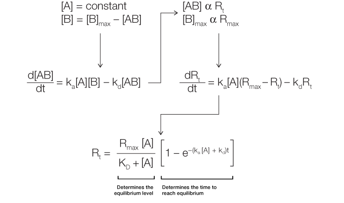
Fig. 2. Derivation of the equation for the association phase.
As can be inferred from this derivation, the change in the amount of complex formed over time is linearly related to ka, kd, and the analyte concentration [A]. The complex formation can be further described in terms of response units, where the change in response units over time is again linearly related to ka, kd, and [A]. Thus, Equation 2 describes the level of response at equilibrium and also the time taken to reach a certain response level during the association phase.
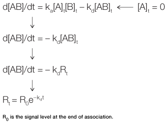
Fig. 3. Derivation of the equation for the dissociation phase.
Dissociation Phase
In the dissociation phase, the analyte concentration in the flow is suddenly reduced to zero by the injection of running buffer. The rate of complex dissociation follows simple exponential decay, or first-order kinetics. Equation 3 is derived in a manner similar to Equation 2. It describes the time taken to reach a certain response level during the dissociation phase, as outlined in Figure 3.
ProteOn Manager software offers two options for the Langmuir model: simultaneous ka/kd and off-rate analysis. The first option is the default choice, which fits both the association and dissociation phases for the full set of constants (ka, kd, and KD), whereas the second option analyzes only the dissociation phase for KD.
Langmuir with Drift or Mass Transport
There are two other kinetic interaction models based on the Langmuir equations: Langmuir with drift and Langmuir with mass transport. Langmuir with drift is commonly used in experiments that use a capture surface, for example, the reversible antibody or histidine-tag capture surface. In such cases the captured ligand may escape from the capture reagent on the chip surface, leading to baseline drift before the analyte injection and during the association and dissociation phases. Note that this model calculates only a linear drift that is constant with time. Blank buffer referencing should be used to improve accuracy when correcting for a large baseline drift showing an exponential curvature.
The second model is Langmuir with mass transport. Mass transport is the process whereby an analyte diffuses from the bulk solution to the chip surface. To determine whether a particular interaction is limited by mass transport and thus whether this model should be used, inject an analyte sample at different flow rates. If the association curves are different, then this interaction is mass transport–limited. In contrast, if the association curves are independent of the flow rate (all binding curves overlap), then diffusion is not the rate-limiting factor, and the simple Langmuir model can be applied.
Other Binding Models
There are four complex binding models for analyzing non-Langmuir interactions: the heterogeneous analyte, heterogeneous ligand, two-state, and bivalent analyte models. When choosing a model to determine the binding kinetics of interactions, the Langmuir or Langmuir with mass transport model should be selected by default since the majority of biological interactions occur in a 1:1 stoichiometry. It is necessary to provide a biological justification for the use of other models, and conclusions based on analyses with these complex models should be confirmed with additional experiments.

Fig. 4. Parameter setting options for kinetic analysis.
Parameter Setting
In ProteOn Manager software, there are two types of parameter setting options for kinetic analysis: (1) under the Fitted heading you can choose Fitted or Constant parameters, and (2) under the Grouped heading you can choose Global, Grouped, or Local sensorgram fitting scopes, as indicated in Figure 4.
The fitted parameters are variables in the sensorgram fitting, whereas constant parameters are fixed at their initial values. The three sensorgram fitting scopes — global, grouped, and local — are defined and compared in Table 1. When setting the parameter fitting types, the initial values of all parameters can be changed to start the sensorgram fitting from a poinr closer to the result. This option may be applied in sensorgram fitting with complex models to reduce computational demands.
Table 1 shows the results of an experiment with the ProteOn protein–small molecule kit. In this experiment, six identical ligand channels were prepared so that the global fitting of all 36 sensorgrams and the grouped fitting of a set of six sensorgrams in each ligand channel are comparable.
Table 1. Results of an experiment using the ProteOn protein–small molecule kit
| Paramater |
ka, Ms-1
|
kd, s-1
|
KD, M
|
Rmax, RU
|
Chi2, RU
|
| Scope |
Global
|
Global
|
Global
|
Global
|
All
|
|
1.51 x 10⁴
|
3.63 x 10⁻²
|
2.41 x 10⁻⁶
|
80.52
|
6.0
|
|
| Scope |
Grouped
|
Grouped
|
Grouped
|
Grouped
|
All
|
| L1 |
1.58 x 10⁴
|
3.76 x 10⁻²
|
2.38 x 10⁻⁶
|
84.9
|
5.3
|
| L2 |
1.60 x 10⁴
|
3.75 x 10⁻²
|
2.35 x 10⁻⁶
|
78.7
|
5.0
|
| L3 |
1.54 x 10⁴
|
3.67 x 10⁻²
|
2.38 x 10⁻⁶.
|
79.3
|
5.1
|
| L4 |
1.54 x 10⁴
|
3.54 x 10⁻²
|
2.30 x 10⁻⁶
|
78.6
|
5.8
|
| L5 |
1.42 x 10⁴
|
3.56 x 10⁻²
|
2.51 x 10⁻⁶
|
80.4
|
5.8
|
| L6 |
1.36 x 10⁴
|
3.48 x 10⁻²
|
2.56 x 10⁻⁶
|
81.3
|
8.1
|
Global: Parameters are identical for all sensorgrams.
Grouped: Parameters are identical for a certain ligand channel.
Equilibrium Analysis
The equilibrium constant, KD, can be calculated directly from a sensorgram using Equation 4:

Equation 4 describes the response at the steady-state or equilibrium phase of the interaction, as shown in Figure 5. In this phase, the rate of association equals the rate of dissociation. To determine the KD, the response at equilibrium, Req, is measured over a given range of analyte concentrations and the values are plotted as shown in Figure 6. Req is proportional to the analyte concentration at the low end of the concentration range, but as the analyte concentration is increased, it approaches the theoretical maximum response Rmax, the limiting value. When performing an equilibrium analysis, use data in which the responses of all analyte concentrations have reached equilibrium and confine the fitted region to the areas where the responses are flat.
Note that in ProteOn Manager software, the equilibrium analysis also presents the choices of fitted or constant and global or grouped for parameter setting. The definitions are the same as those described in the previous section.
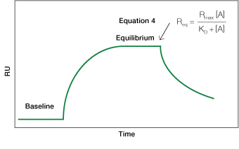
Fig. 5. An idealized sensorgram displaying the equilibrium phase.
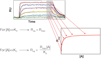
Fig. 6. Determination of the equilibrium constant.
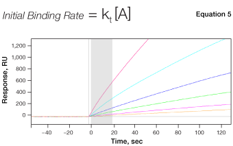
Fig. 7. The mechanism of concentration analysis. kt is the mass transport coefficient in the unit of RU M-1s-1.
Concentration Analysis
Although SPR biosensors can be used to determine analyte concentrations at binding equilibrium in a manner similar to an enzyme-linked immunosorbent assay (ELISA), concentration analysis in SPR biosensors is usually implemented using a different approach for higher efficiency and convenience. Here, the initial binding rate of a biomolecular interaction is measured under mass transport–limited conditions, in which the binding rate is directly proportional to the bulk analyte concentration, as shown in Equation 5. The concentration of an unknown sample is calculated by comparing the binding response under these conditions to a standard curve of binding responses for known concentrations, as shown in Figure 7.
In the ProteOn Manager software, the standard four-parameter logistic equation is employed to determine the unknown concentration. Note that the concentration analysis again presents the scopes of fitted or constant and global or grouped for parameter setting. The definitions are the same as those described in the previous section.
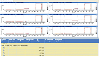
Fig. 8. Report point values are shown in a new column of the data table.
Report Point
A report point is created to directly read the average value of sensorgrams within a specified time range. Sensorgram fitting is not involved in this procedure. A report point is often used to measure the immobilization level of ligands or qualitatively compare the responses with different analyte injections. A report point is created in two steps: (1) right-click and drag to select a time range, and (2) right-click the selected time range to create a report point. The report point values are shown in a new column of the data table, as shown in Figure 8. The report point created in another dataset may be imported to the current dataset by right-clicking the data table and choosing Add Report Point.
Data Presentation
ProteOn Manager software presents the results of an interaction analysis as a data table. The data table shows all the fitted parameters by default. The parameter list can be changed by dragging the parameter columns in or out of a parameter database Column Chooser to customize the parameter list. Right-clicking the data table will bring up this option in the pop-up menu.
The data table is automatically grouped in the same way as the sensorgram sets (typically by ligand channels) and may be ungrouped to display all the values, as shown in Figure 9. In addition, the data table panel can be resized by clicking the arrow buttons at the top-left corner. The values in the data table can be selected and copied to spreadsheets.
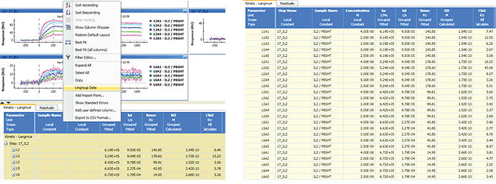
Fig. 9. The grouping and ungrouping of the data table.
In drug discovery research, isoaffinity and screening graphs are frequently used to view the screening results for positive-hit pickup. ProteOn Manager software can be used to create either graph. In the Analysis menu, choose Isoaffinity Graph or Screening Graph to display the graph. Both graphs allow the selection of target datasets in the left panel. Examples of an isoaffinity graph and a screening graph are presented in Figure 10.
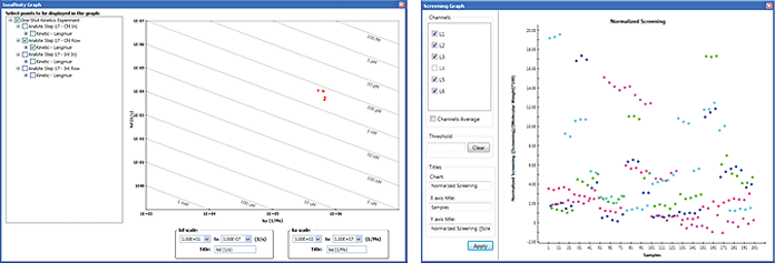
Fig. 10. Examples of an isoaffinity graph (left) and a screening graph (right).
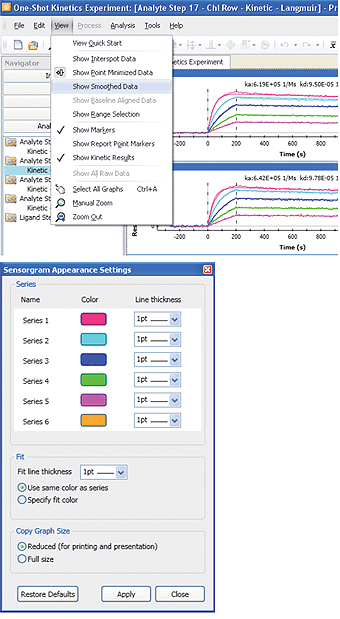
Fig. 11. The sensorgram smoothing and sensorgram appearance setting functions in ProteOn Manager software.
Note: Please refer to the appendix for the different options of exporting SPR results to external software platforms from ProteOn Manager software.
Sensorgram Appearance
To customize the sensorgram visualization to meet user preferences, ProteOn Manager software offers two appearance functions: sensorgram smoothing and sensorgram appearance setting.
Sensorgram smoothing is available in the View menu and may be removed by deselecting it. This function smoothes the baseline noise to better display the curvature of sensorgrams. Note that the sensorgram smoothing is only a display-related feature. It does not affect sensorgram fitting or SPR results because data analysis is always based on the raw data.
The sensorgram appearance setting is available in the Tools menu and allows the user to choose sensorgram color and line thickness. The appearance change will be applied to the sensorgram series (a particular sensorgram in all sensorgram sets) rather than to a single sensorgram. To change the color of a single sensorgram, open the Interaction screen in the Data tab, and right-click an interaction spot to select a color. The sensorgram appearance functions in ProteOn Manager software are shown in Figure 11.
Quality Standards for SPR Results
The following standards are used to judge the quality of SPR results. An example of high-quality SPR results is shown in Figure 12 as a reference for applying the standards.
Visual inspection — the lines of the resulting fit should pass through the experimental sensorgrams. Both the fitted and original data should be displayed for publication.
Parameter results — fitted parameters should be within an expected and reasonable range. The Rmax value should be within the range of a few hundred RU, ideally less than 200 RU, to minimize the impact of mass transport effects. ProteOn Manager software provides the choices of global, grouped, or local sensorgram fitting. When available, it is recommended to compare the results of global and grouped analyses to demonstrate the reliability of the sensorgram fitting. If it is possible to perform both kinetic and equilibrium analyses on the same dataset, the calculated KD value obtained from the equilibrium analysis should be similar to the KD value calculated from the individual ka and kd values obtained from the corresponding kinetic analysis. These two comparisons are usually applied to determine the confidence level of the fitted parameters. The fitting parameters must be recorded when publishing SPR results.
Chi2 — Chi2 is the average of the squared residuals (the average of the squared differences between the measured data points and the corresponding fitted values). The lowest value that can be expected is the baseline noise. The Chi2 value should also be published, as it indicates the fitting confidence. Empirically, these values should be less than 10% of Rmax regardless of units.
Residuals — a plot of the residuals should form a random scattering of the same order of magnitude as the noise level. It is helpful to display the residual data along with the fitted data when publishing your work.
Standard errors — standard errors determine how sensitive the sensorgram fitting is to changes in the parameters and should be included in publications.
Signal-to-noise ratio — the responses in both the association and dissociation phases must show an adequate signal-to-noise ratio (SNR), typically an SNR over 3. Given the fact that the baseline noise is ~1 RU in the ProteOn XPR36 system, the sensorgram rise in the association phase and fall in the dissociation phase must be greater than 3 RU to guarantee the quality of the SPR results.

